LightGlue (ICCV20231) is a blazing fast feature matcher capable of finding correspondences between pairs of images, improving upon previous state-of-the-art model architectures such as LoFTR (CVPR20212) and SuperGlue (CVPR20203) in both accuracy and efficiency. Image matching is a paramount task in visual localization, enabling many applications in computer vision and robotics.
In this post, we show how to accelerate LightGlue inference using ONNX Runtime and TensorRT, achieving 2x-4x speed gains over compiled PyTorch, across a variety of batch size and sequence length combinations, as well as enabling inference in language runtimes outside of Python, like C++.

Additionally, we will detail the techniques which enable the ONNX export of the LightGlue model in the first place, along with specific inference optimizations that can be performed. Our main contributions are:
- We reexpress the forward pass of the LightGlue model & corresponding feature extractors into one that facilitates seamless PyTorch-ONNX export, and in particular, surgically modify the operations and order thereof to be fully compatible with symbolic shape inference - a requirement for the ONNX model to be consumed by the Runtime’s execution providers.
- We introduce end-to-end parallel batch support to the extractor-LightGlue pipeline, allowing for the export of models with dynamic batch sizes.
- We implement attention subgraph fusion (a graph optimization that currently only supports a growing number of transformer architectures like BERT and Llama) for LightGlue to take advantage of the contrib MultiHeadAttention node when running on ONNX Runtime’s CPU and CUDA execution providers.
All models and code are available at fabio-sim/LightGlue-ONNX.
Introduction
The general structure of a image matching pipeline with LightGlue consists of:
- A feature extractor, which takes an image as input and predicts a set of keypoints (expressed as \(x,y\) coordinates) alongside confidence scores and descriptors for each keypoint. A descriptor can be thought of as a vector embedding that describes a keypoint.
- A matcher (in our case, LightGlue) that, given two sets of keypoints and descriptors from two images, predicts which keypoints in the first image correspond to which keypoints in the second.

Extractor Model Architecture
Typically, the feature extractor is a convolutional network like SuperPoint 4 or DISK 5, but conventional algorithms like SIFT 6 can also be used to extract keypoints and descriptors from images. For the sake of brevity, we focus on SuperPoint as the extractor for this post.
More concretely, given a tensor of batched images of shape \((B, C, H, W)\), the extractor runs it through a series of convolutional layers and filters (non-maximum suppression, confidence thresholds) to eliminate redundant and low-confidence keypoints, ultimately producing three components:
- keypoints: \([(N_0, 2),\ldots, (N_{B-1}, 2)]\)
- scores: \([(N_0,),\ldots, (N_{B-1},)]\)
- descriptors: \([(N_0, D),\ldots, (N_{B-1}, D)]\)
where \(N_i\) is the number of keypoints detected in the \(i\)-th image, and \(D\) is the descriptor size.
LightGlue Model Architecture
The LightGlue matcher starts off by positionally encoding the detected keypoints, and alongside their descriptors runs it through several transformer layers, before finally predicting the matches and match scores based on a similarity matrix. That is, looking back at the pipeline figure above, given keypoints \((B, N, 2)\) & descriptors \((B, N, D)\) from images on the left, and keypoints \((B, M, 2)\) & descriptors \((B, M, D)\) from images on the right, LightGlue predicts:
- matches: \([(S_0, 2),\ldots, (S_{B-1}, 2)]\)
- match scores: \([(S_0,),\ldots, (S_{B-1},)]\)
where \(S_i\) is the number of detected matches in the \(i\)-th pair of images.
Optimizations
Notice that the outputs of both the extractor and matcher stages are not single tensors, but rather sequences (lists) of tensors. This follows from the fact that the number of detections is data-dependent, i.e., based on the actual content of the input images. In this section, we expand on the optimizations made for ONNX Runtime inference on NVIDIA GPUs.
End-to-end Parallel Batching
Extractor Stage
Having a variable number of keypoints for each image hinders effective batching and narrows the possibility of exporting a model that supports dynamic batch sizes. There are a couple of ways one can go about merging the list of tensors \([(N_0, 2),\ldots, (N_{B-1}, 2)]\) into a single unified tensor \((B, N_u, 2)\):
- Padding each tensor up to a constant maximum (for example, \(N_u=\max_{0\le i \le B-1}{N_i}\)), or \(N_u=K\) for some constant \(K\) and truncate the excess entries - naturally, this raises the question of what value to pad with, such that the matcher knows to ignore/mask this later on? No obvious answer comes to mind.
- Removing the source of the variability directly - which is pinpointed to applying the filter threshold on the confidence scores. By skipping this step and always selecting the top-\(K\) entries, the output tensors will have identical shapes and can thus be computed in batch. Relevant excerpt from extractor code:
# Detection threshold removed.
# Batch select top-K keypoints using 2D row-major indexing trick
top_scores, top_indices = scores.reshape(b, h * s * w * s).topk(self.num_keypoints)
top_keypoints = top_indices.unsqueeze(2).floor_divide(torch.tensor([w * s, 1])) % torch.tensor([h * s, w * s]).flip(2)
We adopt the second design because it also means that we can compute the extractor forward pass for both left and right image batches in one go, specifically by interleaving left-right images into a single tensor of shape \((2B, C, H, W)\), outputting:
- keypoints: \((2B, N, 2)\)
- scores: \((2B, N)\)
- descriptors: \((2B, N, D)\)
LightGlue Stage
As a result of the previous, the inputs to the LightGlue matcher now have predictable shapes. This allows us to, following the interleaved batch convention above, feed the combined keypoints and descriptors to LightGlue directly, rather than having to separate them into left and right batches.
Recall that LightGlue outputs the matches as a list of tensors too \([(S_0, 2),\ldots, (S_{B-1}, 2)]\), similar to the original extractor. We can also apply a simple trick here, in order to have LightGlue output a unified tensor. Instead of looping over the batch dimension and constructing a list, we exploit advanced indexing so as to output:
- matches: \((S_0+\ldots+S_{B-1}, 3)\)
- match scores: \((S_0+\ldots+S_{B-1},)\)
where matches[:, 0] indicates the batch index of the match. Modified filtering function:
def filter_matches(scores: torch.Tensor, threshold: float):
    """obtain matches from a log assignment matrix [BxNxN]"""
    max0 = torch.topk(scores, k=1, dim=2, sorted=False)  # scores.max(2)
    max1 = torch.topk(scores, k=1, dim=1, sorted=False)  # scores.max(1)
    m0, m1 = max0.indices[:, :, 0], max1.indices[:, 0, :]

    indices = torch.arange(m0.shape[1], device=m0.device).expand_as(m0)
    mutual = indices == m1.gather(1, m0)
    mscores = max0.values[:, :, 0].exp()
    valid = mscores > threshold

    b_idx, m0_idx = torch.where(valid & mutual)
    m1_idx = m0[b_idx, m0_idx]
    matches = torch.concat([b_idx[:, None], m0_idx[:, None], m1_idx[:, None]], 1)
    mscores = mscores[b_idx, m0_idx]
    return matches, mscores
Symbolic Shape Inference Compatibility
In order to be consumed by ONNX Runtime’s execution providers such as TensorRT, it is necessary for the ONNX model to have all shapes be well-defined. However, if one were to naively export the unmodified implementation, shape inference will not work. We highlight the required modifications that must be applied for shape inference to succeed:
flatten()andunflatten()operations, which are commonly implemented in transformer layers (e.g., before and afterscaled_dot_product_attention()), are designed to work for tensors of arbitrary rank. Unfortunately, this often leads to shape inference incorrectly guessing the rank of intermediate tensors and erroring out. To fix this, we reexpress these operations as the stricterreshape(), which has better defined input and output shapes.- Negative indices in
axisordimparameters of operations such asstack(),concat(), andtranspose(), coupled with the previous point, exacerbate the shape inference errors. Therefore, we changed the models to only use non-negative indices for those parameters. Although this is not truly equivalent to the negative-indices version, since the former counts from the start while the latter counts from the end, for tensors of the same rank, they are identical operations. - Additionally, by carefully reordering several operations, we can actually reduce the number of attention function calls in each transformer layer from 4 to 2 and obtain a simpler exported graph.
Attention Subgraph Fusion
Attention fusion is a graph optimization that can be applied by ONNX Runtime to transformer-family models like BERT and Llama. However, in order for this optimization to be applicable, an exact match of not only the attention subgraph but also the downstream nodes like LayerNormalization is compulsory. Fortunately, thanks to the Custom Operators feature in PyTorch 2.4 7, we devise a way to intercept the attention operation during export, thus eliminating the need for tedious subgraph pattern matching. Recall that the attention computation boils down to the following operations:

Ideally, we would like to fuse this subgraph into a single optimized MultiHeadAttention node that is available as a contrib operation in ONNX Runtime. By leveraging the torch.library API, we can intercept this operation during export using the following code snippet:
import torch
import torch.nn.functional as F
from torch.onnx import symbolic_helper

CUSTOM_OP_NAME = "fabiosim::multi_head_attention"

@torch.library.custom_op(CUSTOM_OP_NAME, mutates_args=())
def multi_head_attention(q: torch.Tensor, k: torch.Tensor, v: torch.Tensor, num_heads: int) -> torch.Tensor:
    b, n, d = q.shape
    head_dim = d // num_heads
    q, k, v = (t.reshape((b, n, num_heads, head_dim)).transpose(1, 2) for t in (q, k, v))
    return F.scaled_dot_product_attention(q, k, v).transpose(1, 2).reshape((b, n, d))

@symbolic_helper.parse_args("v", "v", "v", "i")
def symbolic_multi_head_attention(g, q, k, v, num_heads_i):
    return g.op("com.microsoft::MultiHeadAttention", q, k, v, num_heads_i=num_heads_i).setType(q.type())

torch.onnx.register_custom_op_symbolic(CUSTOM_OP_NAME, symbolic_multi_head_attention, 9)

Performance Results
Reproducibility: All measurements are of the full end-to-end matching pipeline (SuperPoint+LightGlue) on an i9-12900HX CPU and RTX4080 12GB GPU. Relevant framework versions: torch==2.4.0+cu121, onnxruntime-gpu==1.18.1, CUDA 12.1, cuDNN 9.2.1, TensorRT 10.2.0.post1. We use the torch.compile()-d model as the baseline, running full layers with mixed-precision & Flash Attention enabled and adaptive depth & width disabled.
The charts below illustrate the speedup gains and overall throughput in image pairs per second for each tested input combination.

From the results, we observe that the TensorRT execution provider is overwhelmingly the fastest out of all options, attaining performance gains of up to 4x. We configure TensorRT to enable FP16 precision in the execution provider options and leave everything else to the defaults. Nonetheless, it is worth noting that TensorRT has an inherent limitation 8 on the maximum number of keypoints that can be extracted (3840). On the other hand, the CUDA execution provider roughly matches the performance of the PyTorch implementation at small numbers of keypoints, but gradually becomes slower at higher sizes.
Future Work
In this post, we considered the LightGlue model without adaptive depth or width, despite it being one of LightGlue’s main strengths. As the TorchDynamo ONNX exporter matures to handle control flow operations like torch.cond(), we expect that it will become feasible to export the adaptive version of LightGlue.
References
-
Philipp Lindenberger, Paul-Edouard Sarlin, Marc Pollefeys; “LightGlue: Local Feature Matching at Light Speed” in Proceedings of the IEEE/CVF International Conference on Computer Vision (ICCV), 2023, pp. 17627-17638. ↩
-
Jiaming Sun, Zehong Shen, Yuang Wang, Hujun Bao, Xiaowei Zhou; “LoFTR: Detector-Free Local Feature Matching With Transformers” in Proceedings of the IEEE/CVF Conference on Computer Vision and Pattern Recognition (CVPR), 2021, pp. 8922-8931. ↩
-
Paul-Edouard Sarlin, Daniel DeTone, Tomasz Malisiewicz, Andrew Rabinovich; “SuperGlue: Learning Feature Matching With Graph Neural Networks” in Proceedings of the IEEE/CVF Conference on Computer Vision and Pattern Recognition (CVPR), 2020. pp. 4938-4947 ↩
-
Daniel DeTone, Tomasz Malisiewicz, Andrew Rabinovich; “SuperPoint: Self-Supervised Interest Point Detection and Description” in CVPR Deep Learning for Visual SLAM Workshop, 2018. ↩
-
Michał J. Tyszkiewicz, Pascal Fua, Eduard Trulls; “DISK: Learning local features with policy gradient” in Advances in Neural Information Processing Systems, vol. 33, 2020. ↩
-
David G. Lowe; “Distinctive Image Features from Scale-Invariant Keypoints” in International Journal of Computer Vision, vol. 60, 2004, pp. 91-110. ↩
-
PyTorch Contributors; “PyTorch Custom Operators”, Accessed 2024. Available: URL ↩
-
NVIDIA, “TensorRT Operators Documentation: TopK”, Accessed 2024. Available: URL ↩